Cluster Messy Time Series

When clustering data, it can be challenging to handle time series data, especially when the series have differing lengths. This lesson contains the code and theory to cluster your own messy time series. You can download the notebook with code here.

Data is messy and contains time series features. How can you extend our clustering toolbox to handle these messy time series tables?

Cluster Time Series Data

When using the k-means algorithm for clustering numerical data, data samples are treated as vectors and the goal is to sort them into k groups, or clusters. A cluster’s archetype is a hypothetical data point that best represents all data assigned to that cluster. Assuming we have an initial guess for the k archetypes, here are the next steps:

Assign data samples to the nearest archetype
Update the k archetypes to be their samples’ center
Iterate this process until the archetypes converge

For k-means, nearest and center are governed by the choice to use Euclidean distance (or square root of the sum of squared distances). This is clear for the “assign” stage; centering via the sample mean is equivalent to minimizing the total Euclidean distance from the archetype to each sample.

When we use absolute distance instead, we get the k-medoids algorithm. As we think about how to cluster our time series data, a natural question arises. What distance metric is well-suited for handling time series?

Earth mover’s distance

One option is the Wasserstein (earth-mover’s) distance metric.

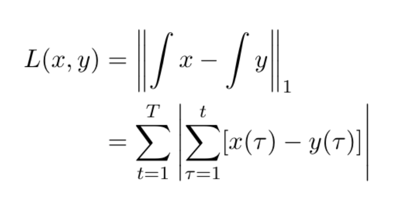
For one-dimensional sequences, we can interpret earth mover’s distance to be the Euclidean distance between the integral (cumulative sum) of two series.

Using the earth mover’s distance is both computationally and intuitively convenient. First, it requires only a single transformation (taking the integral or cumulative sum) before applying the familiar k-means algorithm, and finally deriving the archetypes to return to our original space. Intuitively, comparing integrals is how we measure the differences in shape of time-invariant series.

Handle Time-Varying Lengths

To circumvent the issue of differing lengths of time, let’s imagine that all time series actually have the same length and treat future values as missing. Now the nature of the problem is clustering data with missing values.

There are two standard approaches for handling missing data, and we’ll share a third approach as well.

Approach 1: Drop incomplete samples
As a first attempt, let’s drop all but the longest time series so we don’t need to fit to data with any missing values.

Approach 2: Substitute column means
Next, let’s compute the average value of entries for each point in time across all samples, and replace the corresponding missing value with the average entry from known samples.

Approach 3: New approach
Finally, we have a third method to initialize our archetypes. We proceed as we did on our first attempt, but then incorporate data with fewer and fewer entries into the archetype estimation process without adding or injecting any made-up data.

Clustering messy data tables

So far, we’ve limited our scope to tables that only have one time series feature. With additional features, it becomes possible to guess what a time series would be if it were actually observed. But, we can leverage the sample’s other features and the patterns captured across the rest of the data to make a prediction.

We refer to this as time series imputation. This approach helps us estimate how valuable a customer would be upon conversion. If we were looking at stocks, it could help us estimate how valuable a company would be after an IPO.

Algorithm and Approach

Here is the best method for handling time-varying time series. It works even when the time series are all missing future values, i.e., right-ward entries for each sample’s relative sense of the present. It will also work for larger tables where additional data has numeric features. We use the Euclidean metric to measure distance for these.

Pivoted clustering algorithm:

Drop samples where any entries are missing
Cluster using a variation of k-means
Collect samples that are missing last time entry
Assign these samples to centroids while ignoring missing features
Update centroids for a subset of features to reflect additional assignees
Repeat steps 3-5 for the next missing entry until all samples are clustered

Even messier data

Beyond these examples, it’s important to note that not all features will be numeric and time series may not have missing values in a highly structured way. When this is the case, we can no longer use our pivoted clustering algorithm.

Fortunately, the third algorithm is a simplified case of a more general framework called Generalized Low Rank Models (GLRMs). You can use this framework to cluster messy data and across more general applications.