
In the past 60 years, numerous Buy Til You Die (BTYD) methods have tackled the customer lifetime value problem. BTYD models fit probabilistic models to historical transaction data to calculate CLV., and these models can help answer numerous questions, including:
- How many customers are active?
- How many customers will be active one year from now?
- Which customers have churned?
- How valuable will any customer be to the company in the future?
Strengths
What unites BTYD models is the customer-level treatment of random events like churn, event timing, and order value. In particular, the time (say, weeks) between events (often called the intra-transaction time or ITT) is drawn from a family of parameterized distributions that is personalized to each customer. Meanwhile, customer churn is drawn from its own parameterized and personalized distribution.
A persistent challenge is the lack of data for new and recent customers. In cases like this, Bayesian statistics point to the use of cohort-level patterns as priors for customer-level parameters. This balance of cohort patterns against sparse customer evidence is referred to as customer heterogeneity.
Over the decades, many variations have quantified the value of new flexibilities, relaxed assumptions and speedier algorithms.
History
The different BTYD model implementations include:
- NBD (Ehrenberg 1959)
- Pareto/NBD Schmittlein, Morrison, and Colombo 1987)
- BG/NBD (P. Fader, Hardie, and Lee 2005)
- Pareto/NBD (HB) Ma and Liu (2007)
- MBG/NBD Batislam, Denizel, and Filiztekin (2007), Hoppe and Wagner (2007)
- Pareto/NBD (Abe) Abe (2009)
- BG/BB (Fader, Hardie, and Shang 2010)
- Pareto/GGG Platzer and Reutterer (2016)
This is not an exhaustive list, nor does it include some of the more experimental machine-learning based CLV. Rather it captures flavors and variations in BTYD models, which have served as gold standard by academic and business communities for decades.
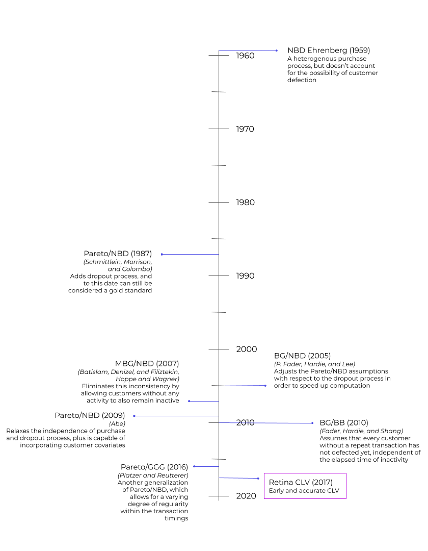
The original NBD model from 1959 functions as a benchmark for later models because it’s based on a heterogenous purchase process. But, NBD doesn’t account for customer churn.
The next model, Pareto/NBD from 1987, adds a heterogeneous dropout process and is considered one of the top buy-til-you-die models.
Next up, the BG/NBD model adjusts assumptions to reduce computation time and offers a more robust parameter search. However, this model assumes customers without repeat transactions have not churned.
MBG/NBD removes inconsistencies with the former model by allowing customers without any activity to remain inactive.
The newer BG/CNBD-k and MBG/CNBD-k models improve forecasting accuracy by allowing for regularity in transaction times. If this regularity exists, these new models can result in much more accurate customer-level predictions.
The variants of Pareto/NBD models by Ma and Liu (2007) and by Abe (2009) utilize MCMC simulation to allow for more flexible assumptions. The first model, Pareto/NBD (HB) is a hierarchical Bayes variant that tests out this approach while sticking to the original model’s assumptions. The second variation, Pareto/NBD (Abe), can incorporate covariates.
Pareto/GGG is a third variation of Pareto/NBD that accounts for some level of regularity for inter-transaction times.
Drawbacks
These BTYD models are elegant and powerful, yet suffer from crippling algorithmic complexity (for 1+ million customers) in all but the most special cases. Where possible, maximum likelihood point-estimate (MLE) solutions are fast, but their accuracy usually underperforms against Monte Carlo Markov Chain (MCMC) simulations which are notoriously slow and expensive to generate. What’s more, BTYD models are loaded with parametric-family assumptions, a hallmark of Bayesian paradigms.