In this lesson, we’ll share a popular method for calculating CLV using the R programming language. A similar lesson in Python can be found here.
To prepare for this exercise, you’ll need:
- An R environment (such as RStudio)
- The BTYDPlus package
- The CDNow dataset
Follow along to predict future spend at the customer level using a Bayesian Buy Til You Die (BTYD) approach, the Beta-Geometric negative binomial distribution (NBD) CLV model.
Load in the data
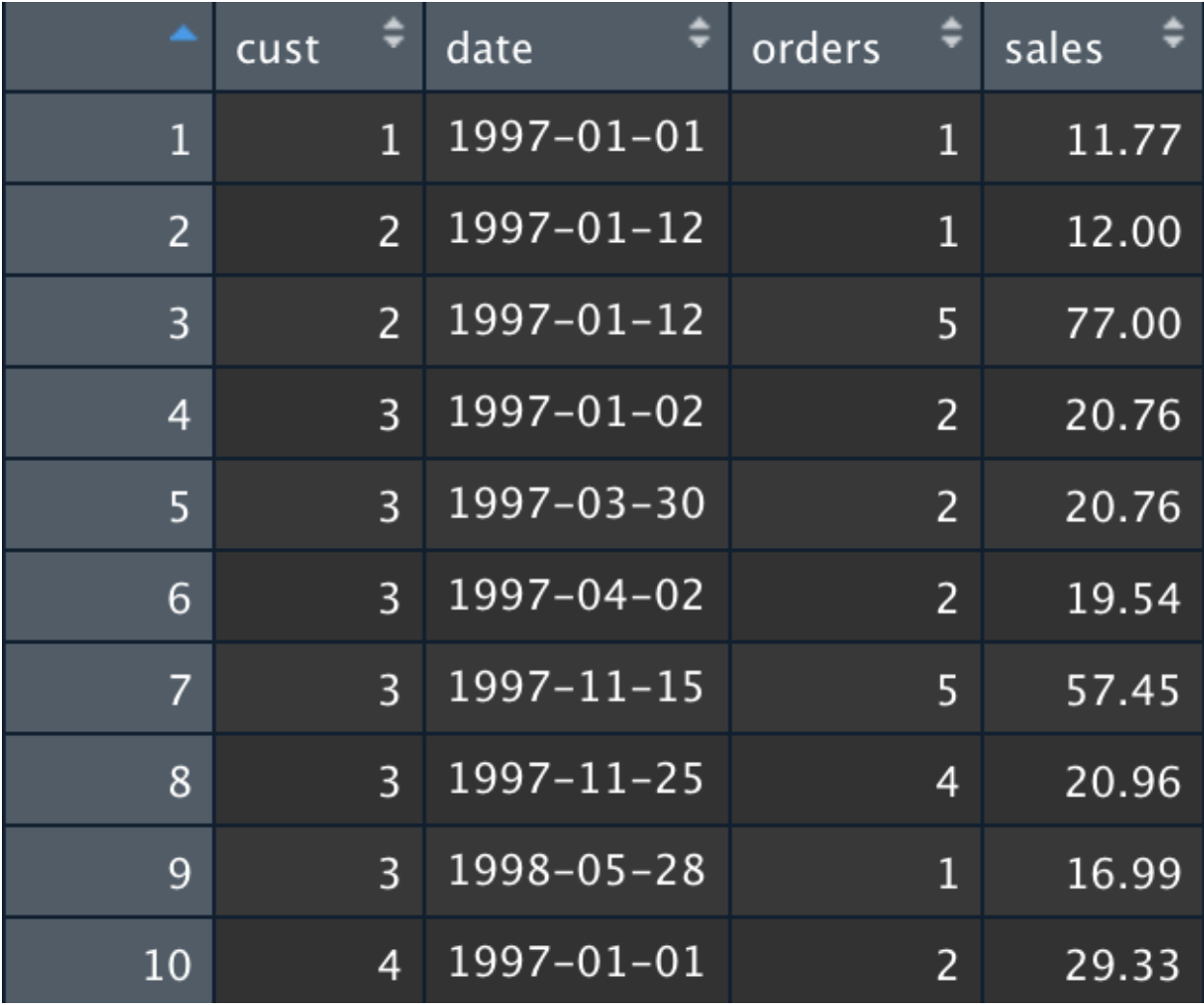
The data comes in a .txt file that we can use R’s read.table to parse. We’ll also need to do some renaming of columns and reformatting of dates.
data <- read.table('CDNOW_master.txt', sep = "" ,
header = F , nrows = 69659,
na.strings ="", stringsAsFactors= F)
colnames(data) <- c('cust', 'date', 'orders', 'sales')data$date
<- as.Date(as.character(data$date), format='%Y%m%d', origin="1970-01-01")
Once the data is loaded in, it should look like this:
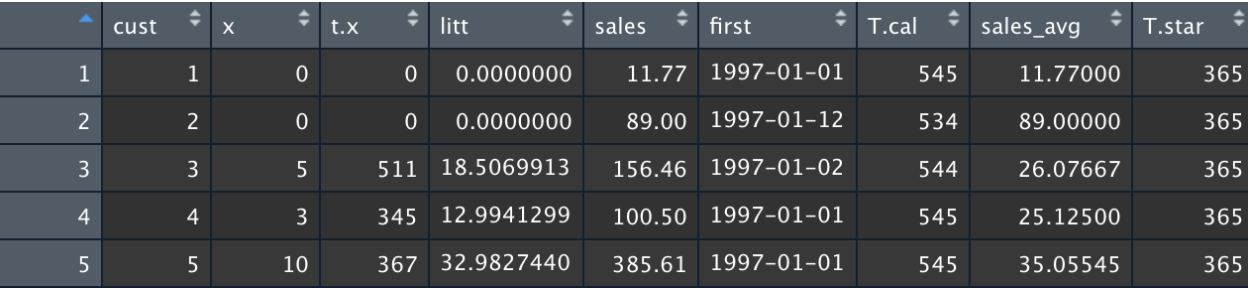
Aggregate into customer-level parameters
We can use one of the built in functions in BTYDplus to help us change this orders-level data into customer-level data. This function converts the orders data into ITT (Intra-Transaction Time) and total sales data for each customer.
Next, let’s compute the average order size for each customer using the total sales and the number of orders. Finally, set the prediction horizon (T.star) to one year (365 days) for everyone. If we want to predict future spend across a different length of time, we can just change T.star.
library(BTYDPlus)
customer_rdf <- BTYDplus::elog2cbs(
data,
unit = 'days',
T.cal = max(data$date),
T.tot = max(data$date)
)
customer_rdf$sales_avg = customer_rdf$sales / (customer_rdf$x + 1)

bgnbd_rdf <- customer_rdf
bgnbd_rdf$T.star <- 365
The resulting customer data table looks like this:
Call the BTYD package using the R dataframe created above
We will use a statistical approach to predict CLV using the BTYD family of models. In this module, let’s use a Beta-Geometric NBD (Negative Binomial Distribution) model. The BTYD family also includes other models that have different strengths and assumptions. (The widely-regarded industry standard for CLV prediction is Pareto NBD.)
This model will use each customer’s spending behavior to predict the number of transactions they’ll make in the chosen time period.
params_bgnbd <- BTYD::bgnbd.EstimateParameters(bgnbd_rdf) # BG/NBD
bgnbd_rdf$predicted_bgnbd <- BTYD::bgnbd.ConditionalExpectedTransactions(
params = params_bgnbd,
T.star = bgnbd_rdf$T.star,
x = bgnbd_rdf$x,
t.x = bgnbd_rdf$t.x,
T.cal= bgnbd_rdf$T.cal
)
Calculate CLV
Once we have the predicted number of transactions, we can compute CLV by multiplying the predicted number of transactions by the average monetary value (spend).
bgnbd_rdf$predicted_clv <- bgnbd_rdf$sales_avg * bgnbd_rdf$predicted_bgnbd
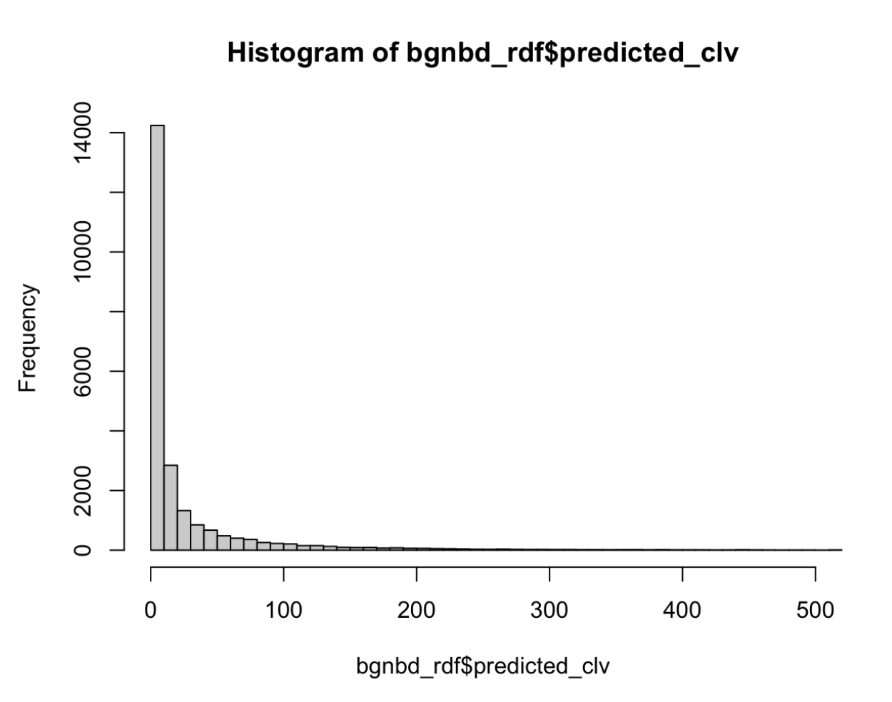
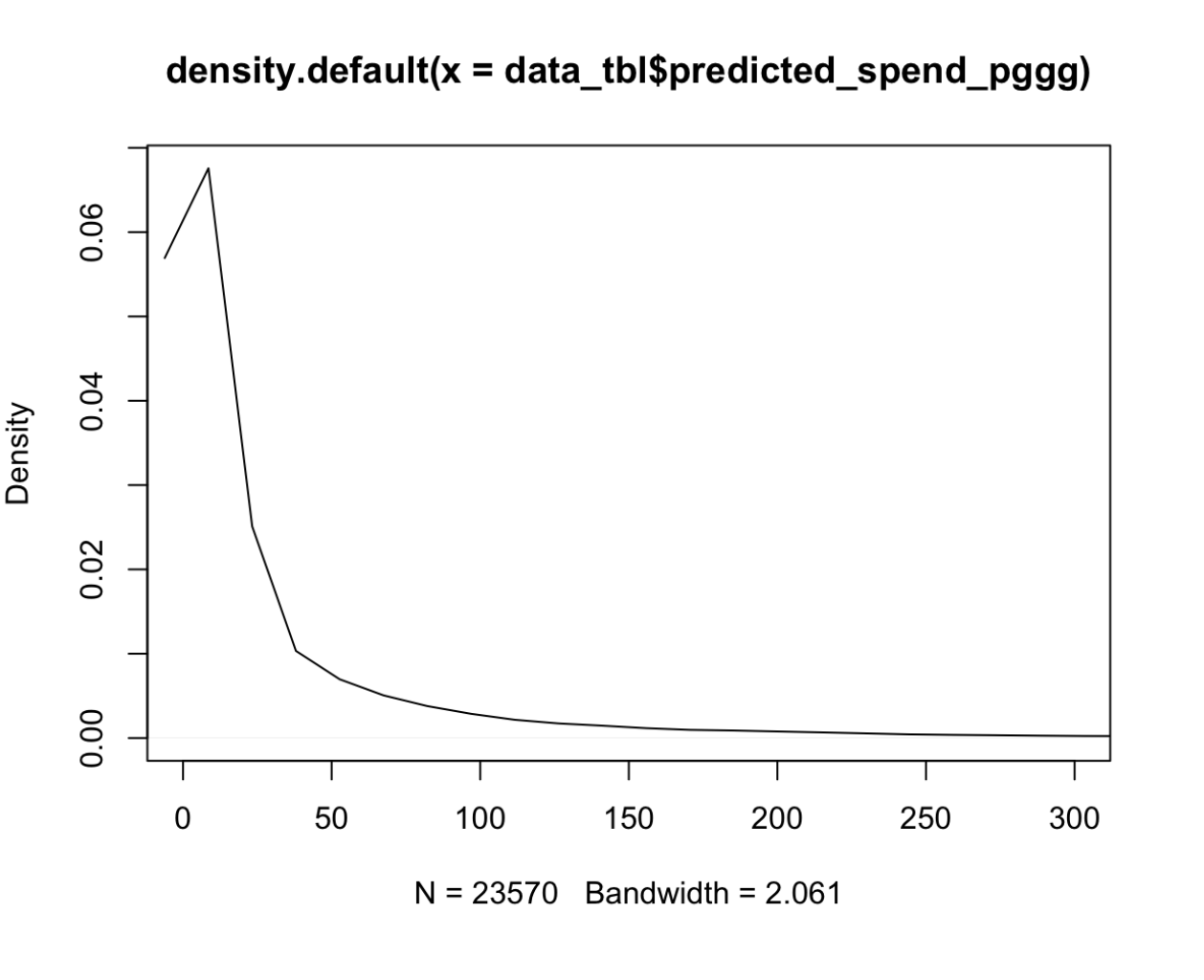
Visualize the CLV results
hist(bgnbd_rdf$predicted_clv, xlim=c(0,500), breaks=3000)
plot(density(bgnbd_rdf$predicted_clv), xlim=c(0,300))
Fortunately the package is equipped with figures, plots and methods to help you visualize and understand the results. We’ve shared some here and hope you can explore on your own, too.