
How much is each one of your customers worth? How much should you spend to acquire them? What about to retain them?
Customer lifetime value (CLV) is the metric leading companies use to understand their customers’ purchasing habits. Simply put, customers who purchase higher-value products, who purchase more frequently, and who continue to purchase on an ongoing basis are your high-CLV customers. That means the total CLV of all of your customers then represents both the realized and future value of your business, so it’s an essential metric for assessing business health.
But how do you determine the CLV for each one of your customers? In this post, we describe three leading approaches to this problem using code snippets and an accompanying Jupyter Notebook.
Defining “customer value”
One of the powers of CLV is that it is flexible enough to be applied across a range of business types. Anything that can be represented numerically and tied to an individual customer at a point in time can be predicted via CLV.
At Retina, most of our clients are direct-to-consumer brands, so for them, customer value represents one of the following:
- Gross Revenue
- Net Gross Margin
- Discounted Cash Flow (DCF)
However, “customer value” can also be extended to mean other measures, such as:
- Content Engagement
- Social Media Engagement
- Referral Value
In each case, past customer value is used to predict future customer value.
Setup and Data
We will use Python/Pandas to illustrate these CLV techniques on an example dataset. However, these same techniques can also be used in R.
In this example, we use publicly available CD-ROM purchases from 1997 and 1998 and “customer value” represents gross revenue.
First, we load the order data into a Pandas DataFrame and convert our input data into appropriate data types:
import pandas as pd
import re
from datetime import datetime
# data from http://www.brucehardie.com/datasets
data_path = 'CDNOW_master.txt'
orders_list = []
with open(data_path) as f:
for line in f:
inner_list = [
line.strip()
for line in re.split('\s+', line.strip())
]
orders_list.append(inner_list)
orders = pd.DataFrame(
orders_list,
columns = ['id', 'date', 'orders', 'spend'])
orders['date'] = pd.to_datetime(orders['date'])
orders['spend'] = orders['spend'].astype(float)
orders = orders[orders['spend'] > 0]
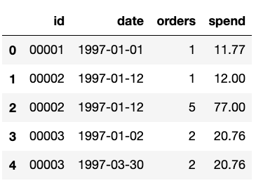
orders.head()
As a result, here are the first 5 rows of our “orders” DataFrame:
Model 1: Analytic Aggregate CLV
Let’s start with the simplest and oldest method for computing CLV, which assumes a constant rate of spend and churn for all customers. In this approach, we define customer lifetime value as:
\[\mbox{CLV} = \bar s / \bar c,\]where \(\bar s\) is the average spend rate and \(\bar c\) is the average churn rate, and averages are taken over customers and time. Both rates must share the same time units in order for the calculation to work.
For simplicity’s sake, this model assumes customers can churn only once and then never purchase again. In expectation, value from one customer at time interval \(i\) will be \(\bar s (1-\bar c)^i\). This represents the expected spend times the probability of not churning for \(t\) intervals. Expected future value is the infinite geometric sum,
\[ \mbox{CLV} = \bar s \displaystyle\sum_{t = 0}^{\infty} \left(1 – \bar c \right)^t, \]which reduces to the equation above.
CLV evaluation requires estimates for average spend \(\bar s\) and churn \(\bar c\). Clearly, population averages provide data-driven approximations for these. In particular,
\[\bar c = \frac{\sum_{i=1}^m d_i}{\sum_{i=1}^m a_i},\]where \(m\) is the number of customers,
\[ d_i = \left\{ \begin{array}{rl} 1 & \mbox{customer $i$ is dead} \\ 0 & \mbox{otherwise,} \end{array} \right.\]indicates whether customer \(i\) is dead and \(a_i\) is the age of customer \(i\) (number of intervals not dead). This requires a decision rule for labeling customers as dead—for example, if too much time has passed since their most recent purchase. Similarly, average spend
\[\bar s = \frac{\sum_{i=1}^m s_i}{m\sum_{i=1}^m a_i}, \]where \(s_i\) is how much customer \(i\) has spent over the course of their lifetime.
The limitations of this approach come from its assumptions: (1) that spend stays constant over time and (2) that all customers behave the same. Because these assumptions do not hold at an individual customer level, this approach can only be used at the aggregate level. That is, this approach calculates lifetime total value (LTV), which is the lifetime spend of customers in aggregate, rather than individually.
To implement this in code, the first step is to compare their first and last order dates in order to calculate customer age. We use months to measure time because it’s our expectation for the typical interval between purchases.
from datetime import timedelta
from numpy import ceil, maximum
group_by_customer = orders.groupby(
by = orders['id'],
as_index = False)
customers = group_by_customer['date'] \
.agg(lambda x: (x.max() - x.min()))
customers['age'] = maximum(customers['date'] \
.apply(lambda x: ceil(x.days / 30)), 1.0)
customers = customers.drop(columns = 'date')
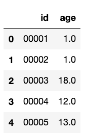
customers.head()
Our table of customer ages looks something like this:
Assuming a customer will never return (has churned) after 12 weeks of inactivity, we use the formulas above to calculate CLV.
twelve_weeks = timedelta(weeks = 12)
cutoff_date = orders['date'].max()

dead = group_by_customer['date'].max()['date'] \
    .apply(lambda x: (cutoff_date - x) > twelve_weeks)

churn = dead.sum() / customers['age'].sum()
spend = orders['spend'].sum() / customers['age'].sum()

clv_aa = spend/churn
print(clv_aa)
As a result, the analytic aggregate CLV model predicts customer CLV to be $123.05 for each customer.
Model 2: Analytic Cohort-based CLV
The next step is to group customers by their cohorts, under the assumption that customers within a cohort spend similarly. Now, we’ll calculate CLV for each cohort:
\[\mbox{CLV}_j = \bar s_j / \bar c, \quad \quad j = 1, \ldots, N, \]where \(N\) is the number of cohorts and \(s_j\) is the average spend rate for cohort \(j\), which can be calculated as follows,
\[\bar s_j = \frac{\sum_{i \in G_j} s_i}{|G_j|\sum_{i \in G_j} a_i}, \]where \(G_j\) is the set of customers assigned to cohort \(j\).
The most common way to group customers into cohorts is by start date, typically by month. The best choice will depend on the customer acquisition rate, seasonality of business, and whether additional customer information can be used. It’s possible to choose cohorts of size 1 and calculate average spend individually, but CLV estimates for customers with very few purchases may be unreliable.
Returning to our coding example we choose cohorts to be singletons for each customer, just for fun.
customers_ac = customers.merge(
    group_by_customer['spend'].sum(),
    on = 'id')

customers_ac['clv'] = customers_ac['spend'] / customers_ac['age'] / churn
customers_ac.head()
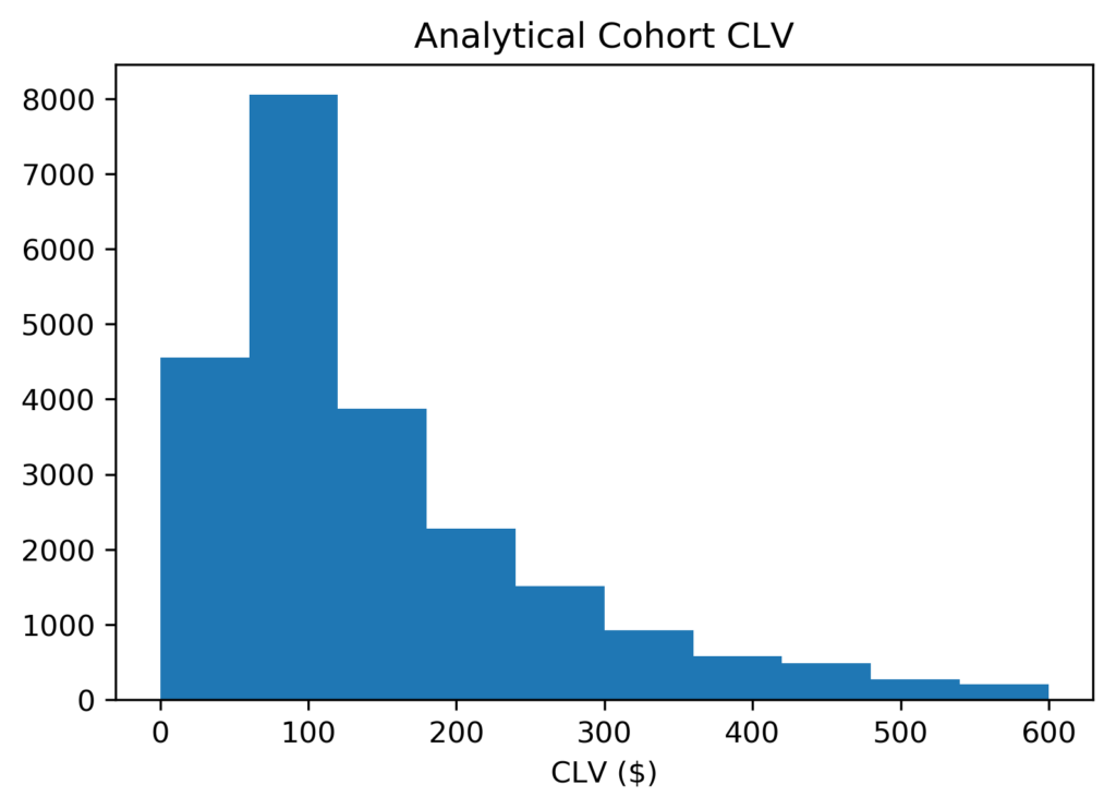
By doing so, each customer has their own CLV prediction. A choice of larger cohorts would produce a CLV estimate for each cohort.
A histogram of CLV predictions shows that most fall between $5 and $600, and the mostly likely prediction is a little less than $100. Finally, the mean is $174.66 and the median is $105.67.
Model 3: Predictive CLV using statistical models
In the final approach for this blog, we consider that individuals differ in churn as well as spend. While the concept appears simple, we must now fit a hierarchical statistical model in order to calculate CLV. This class of models is known as “Buy Til You Die” (BTYD), because the model learns to predict how long a customer will continue to purchase until they churn.
Specifically, a BTYD model will fit a statistical model to predict the number of transactions by customer, then fit a secondary model to predict revenue for any transaction.
Fortunately, training these models to learn from data is straightforward if you use the Lifetimes package in Python. This package uses the “Pareto/NBD” model. Note that this is just one of many available BTYD models, and others may perform better on your data.
To prepare our data for this model, we calculate the recency, frequency, and age for each customer:
from lifetimes.utils import summary_data_from_transaction_data
data = summary_data_from_transaction_data(
orders, 'id', 'date',
monetary_value_col='spend',
observation_period_end = cutoff_date)
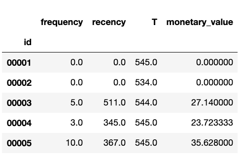
data.head()
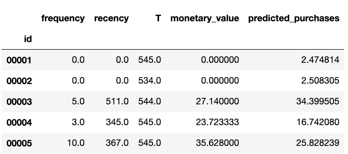
Here are some rows that result from this customer summary table:
Now we fit a Beta-Geometric model to the data,
from lifetimes import BetaGeoFitter

bgf = BetaGeoFitter(penalizer_coef=0.0)
bgf.fit(data['frequency'], data['recency'], data['T'])
to predict the number of transactions expected from each customer over the course of their lifetime.
future_horizon = 10000
data['predicted_purchases'] = bgf.predict(
    future_horizon,
    data['frequency'],
    data['recency'],
    data['T'])
data.head()
Our new customer table now includes lifetime predicted purchases:
To map this back to CLV, we must estimate revenue for each transaction by fitting spend data to Gamma-Gamma model:
from lifetimes import GammaGammaFitter

returning_customers_summary = data[data['frequency'] > 0]

ggf = GammaGammaFitter(penalizer_coef = 0)
ggf.fit(
    returning_customers_summary['frequency'],
    returning_customers_summary['monetary_value'])
transaction_spend = ggf.conditional_expected_average_profit(
    data['frequency'],
    data['monetary_value']
).mean()
print(transaction_spend)
According to this model, the expected revenue from each transaction is $36.18. Now it’s possible to calculate CLV,
customers_pm = customers_ac.join(
    data['predicted_purchases'],
    on = 'id',
    how = 'left'
).drop(columns = 'clv')

customers_pm['clv'] = customers_pm \
    .apply(
        lambda x: x['predicted_purchases'] * transaction_spend,
        axis = 1)
customers_pm.tail()
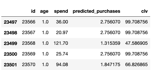
Let’s see how that CLV is distributed:
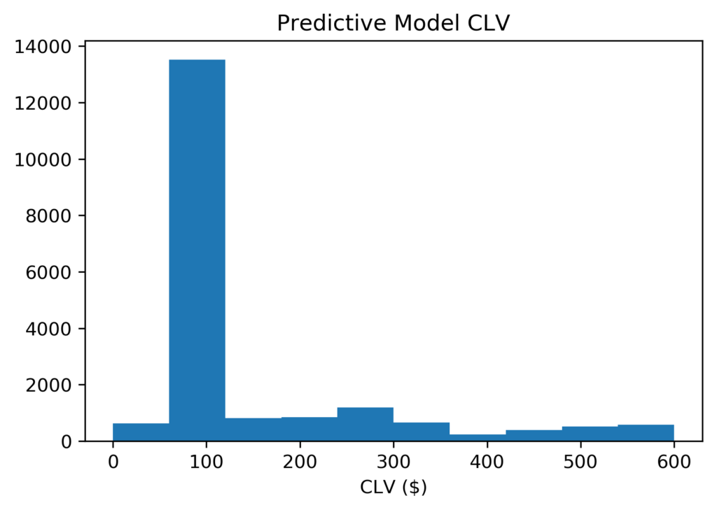
Once again, a histogram shows that most CLV predictions are still between $5 and $600, and the mostly likely prediction is a little less than $100. However, our model is now much more confident that a typical customer will spend about $100. Among customers that spend more, they are almost equally likely to spend $200 or $600. Hence, this rightward skew raises the mean to $424.09 and yet the median remains at $97.81.
Complex Models Can Improve Predictions and Business Outcomes
These three approaches to CLV show that increasing model complexity improves prediction quality. Customer-level and other sophisticated models are pursued by academics and industry researchers. These include the use of Buy Til You Die (BTYD) Bayesian models as well as supervised and unsupervised machine learning models.