
Most traditional BTYD models are Bayesian statistical, meaning the models make parametric assumptions about the R, F, and M components of a CLV model. In this lesson, we’ll explore an alternative way of modeling short-term CLV using Long-Short Term Memory (LSTM) Recurrent Neural Networks (RNNs), which are a type of supervised machine learning that can handle time series well.
In this lesson, we’ll explore traditional approaches, introduce a new one and then compare results from an experiment.
Data
To build a supervised RNN model for CLV, we start with customer transaction history. The dataset we feed into our model might look something like this:
| customer_id | order_id | order_date | order_value |
| 100022 | 100 | 2016-12-21 | 29.00 |
| 100022 | 101 | 2016-12-28 | 36.00 |
| 101046 | 200 | 2018-03-25 | 15.95 |
| … | … | … | … |
We can visualize this with a timing patterns graph:
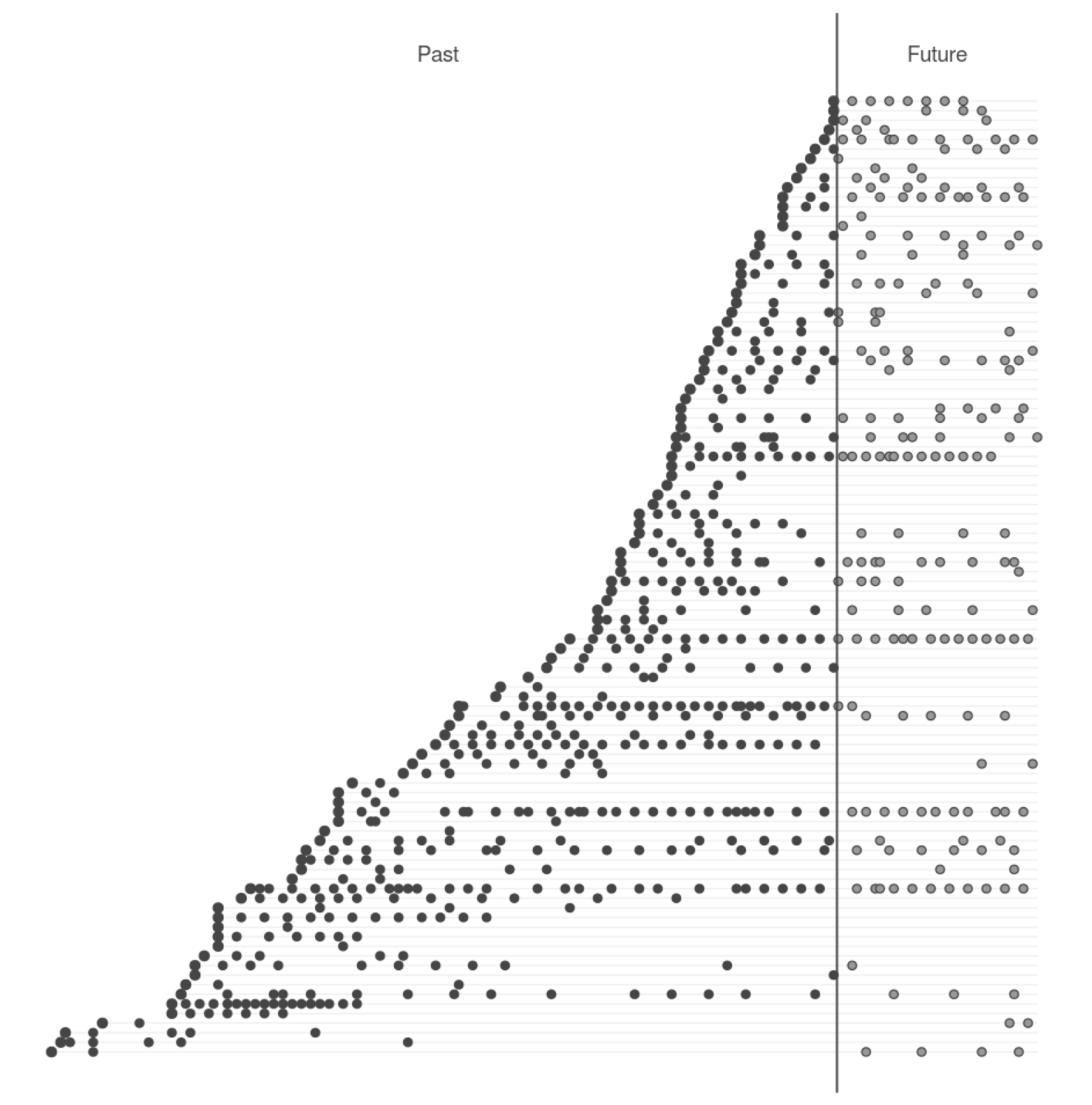
The above graphs shows each historical transaction as well as predicted future transactions:
- The vertical grey line marks today,
- The horizontal grey lines represent individual customers,
- Black dots are transactions in our transaction history,
- Grey dots are transactions predicted by our model.
Assessing a model
But how do we generate these predicted transactions and revenues? And more importantly, how do we know how accurate they are?
First, we split our transaction history data into calibration and holdout datasets. We do so by determining a date that falls somewhere about 80% of the way between the oldest transaction and a more recent transaction in our data set. The transactions that happened before on or before this date are part of the calibration period, and the transactions that happened after are part of the holdout period. These datasets are so named because the calibration period data is fed into the model to calibrate it, while the holdout period data is deliberately withheld to test a model’s prediction ability.
If a model can use the data provided in the calibration period to accurately predict the data in the holdout period, then we know it is a strong model.
Comparing the models
Common models used to calculate CLV are the Pareto/NBD model and the Pareto/GGG model. Pareto/GGG is a powerful CLV model that creates three gamma distributions to determine customer inter-transaction time (ITT) and churn probability. If you’d like to explore it deeper, you can read more about this model in the original paper or the BTYD package.
We have developed a newer model that is being compared against Pareto/GGG today. It’s called the Long-Short-Term-Memory Recurrent Neural Network model (RNN-LSTM). This model takes in a sequence of events and looks for patterns in those events leading up to the present, which allows it to predict the future. We feed the model with customer transaction history hoping it will learn future transactions in our case.
Results
By using our calibration/holdout technique outlined above, we were able to see the prediction strength of each of our models. We also included additional Pareto family models (BG/NBD and NBD) to provide context to our results. So, here are the results from our experiment:
| Model | Total # of Holdout Transactions | Deviations for Actual (#) | Deviation from Actual (%) | Mean Absolute Error (MAE) |
| Actual | 28,224 | n/a | n/a | 0 |
| Pareto/GGG | 28,749 | +525 | 1.9% | 1.56 |
| RNN-LSTM | 26,456 | -1,768 | 6.3% | 1.62 |
| BG/NBD | 28,733 | +509 | 1.8% | 1.70 |
| Pareto/NBD | 28,382 | +158 | 0.6% | 1.75 |
| NBD | 39,619 | 11,395 | 40% | 2.33 |
When we compare the actual number of transactions in our holdout period to the number each model predicted, we can see how well each model fared. The above table is sorted by Mean Absolute Error (MAE), or the average per customer difference between the predicted number transactions and the actual number of transactions.
With the exception of NBD, the statistical models all performed strongly (less than 10% deviation from true values) on this metric. This means they are able to successfully capture customer purchasing trends at the aggregate level. Interestingly, our RNN-LSTM model is the only model that underestimates the total number of holdout transactions.
The figure compares the accuracy of both RNN-LSTM and Pareto/GGG across different purchasing amount per customer:
What this chart demonstrates is that RNN-LSTM underpredicts churned customers (customers who did not purchase anything in the holdout period) and over-predicts others. Pareto/GGG also underpredicts churned customers and overpredicts 3-4 purchase customers, but to a lesser degree.
Discussion
At Retina, we have tried using a variety of models to predict customer lifetime value. In this lesson, we compared the results to evaluate the prediction strength of each model using our calibration/holdout technique.
As we see when comparing performance, Pareto/NBD performs worse on an individual level than Pareto/GGG and RNN-LSTM. In this case, we didn’t see a lot of success with LSTM for predicting CLV.
At Retina, we explore how well we can predict CLV with more recent machine learning models. While we didn’t see a lot of success with LSTM-RNNs in this case, we’ve seen better performance using semi-supervised approaches. Read more about our framework for CLV in this whitepaper.